Background

Basis splines were invented by developed by I.J. Schoenberg and made numerically stable by Carl de Boor for the parametric representation of curves, surfaces, volumetric data, etc. The are more commonly known as B-splines.

One dimension

The basis

As the name suggests, B-splines are constructed as a linear combination of basis functions, which are hat-like functions of compact support, i.e. each function is nonzero only in a bounded range. The basis is constructed in such a way as to guarantee the continuity of the value, and perhaps derivatives of the B-spline, depending of the B-spline degree, N. The B-spline basis is determined by two pieces of information:

an ascending sequence of points, or knot values, which are abscissas for the spline function
the B-spline degree, N.

The degree determines how smooth the spline will be. For degree N, the value and first N-1 derivatives of the spline function will be continuous. Cubic B-splines (N=3) are perhaps the most common form, and have continuous value, first, and second derivatives.

Uniform case:

In the case of a grid with uniform spacing, the basis functions for a cubic B-spline look like:

The vertical lines show the locations of the knots and the colored lines show the basis functions. Note that at any value of x, only four basis functions are nonzero.

Nonuniform case:

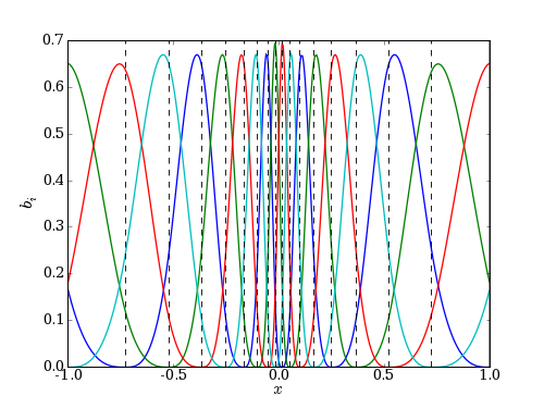
We can also construct a grid with nonuniform spacing. This is useful if the function to be represented has detailed structure concentrated over one part of it's range. For example, the radial wave functions for an atom have rapid oscillations near the nucleus, but are much more slowly varying at large distance. For a nonuniform grid spacing, the basis looks like:

The basis function of degree n centered around grid point i can be given recursively as:

For a specific degree, these can be evaluated quickly without the explicity use of function recursion, as is done in einspline.

Interpolating equations

Once the basis is established, we must solve for the B-spline coefficients. The einspline library chooses the coefficients such that the B-spline interpolates the data, i.e. the B-spline curve passes through the data values given at the knots.
In periodic boundary conditions, these equations may be written in matrix form as

where

.
For fixed first or second-derivative boundary condtions, they take the form

The einspline library solves these equations efficiently using row-reduction and back substitution.

Multi-dimensional B-splines

Tensor-product bases

The one-dimensional B-spline can be generalized to two or more dimensions. To do this, we can construct a two-dimensional basis consisting of the tensor product of one-dimensional basis functions in each direction. For example, for a 1D cubic B-spline, their are four non-zero basis functions at each point, x. In 2D, we construct a 1D basis for x and y separately, then construct the 2D basis as the tensor product and of the x and y basis functions. Thus, for each point in the 2D space, their are 16 nonzero product basis functions. Similarly, in 3D, there are 64 nonzero basis functions which contribute a tricubic B-spline. 4D B-splines could also be constructed, but are not implemented in the einspline library at this time.

The great advantage of B-splines is that the number of floating point value which needs to be stored per mesh point does not increase with dimensionality. In contrast, the more commonly used splines required 2^d floating point values per mesh point. Thus, we save a factor of 8 in storage in 3D. Furthermore, the B-splines can be made to give exactly the same result as standard splines, within numerical round-off error.

A multi-dimensional interpolating B-spline can be constructed solving the interpolating equations for each direction in sequence. That is, for a 2D spline, we first solve the interpolating equations in the x direction for each value of y, using the data to be interpolated, F(x_i, y_j), as the right-hand-sides (RHS) of the equations. This yields of set of coefficients, F^x(x_i, y_j). We then solve the interpolating equations in the y direction, using these F^x coefficients as the RHS, yielding the final 2D B-spline coefficients.